ggplotでヒストグラムを作る geom_histogram()の使い方
Rでggplotを使ってヒストグラムを作る時に使われるのが, geom_histogram()という関数です. ここでは, いくつかの例を元に, その使い方を解説していきます.
geom_histogram()のaes()内で扱える引数
- x
- alpha
- colour
- fill
- linetype
- size
- weight
geom_histogram()の使い方の流れ
ggplotを使うのが初めての方は, 良かったら「ggplotの使い方」を参考にしてください. このページでは, ggplotの関数の中でも, 特にgeom_histogram()関数の使い方の流れを説明していくつもりです.
では, まず一番シンプルなヒストグラムを作成してみます. 使用するデータセットはirisです.
> library(ggplot2)
> str(iris)
'data.frame':	150 obs. of  5 variables:
 $ Sepal.Length: num  5.1 4.9 4.7 4.6 5 5.4 4.6 5 4.4 4.9 ...
 $ Sepal.Width : num  3.5 3 3.2 3.1 3.6 3.9 3.4 3.4 2.9 3.1 ...
 $ Petal.Length: num  1.4 1.4 1.3 1.5 1.4 1.7 1.4 1.5 1.4 1.5 ...
 $ Petal.Width : num  0.2 0.2 0.2 0.2 0.2 0.4 0.3 0.2 0.2 0.1 ...
 $ Species     : Factor w/ 3 levels "setosa","versicolor",..: 1 1 1 1 1 1 1 1 1 1 ...
> p <- ggplot(iris, aes(x=Sepal.Length))
> p + geom_histogram()
stat_bin: binwidth defaulted to range/30. Use 'binwidth = x' to adjust this.
> ggsave("geom_histogram1.png")
Saving 7 x 7 in image
stat_bin: binwidth defaulted to range/30. Use 'binwidth = x' to adjust this.
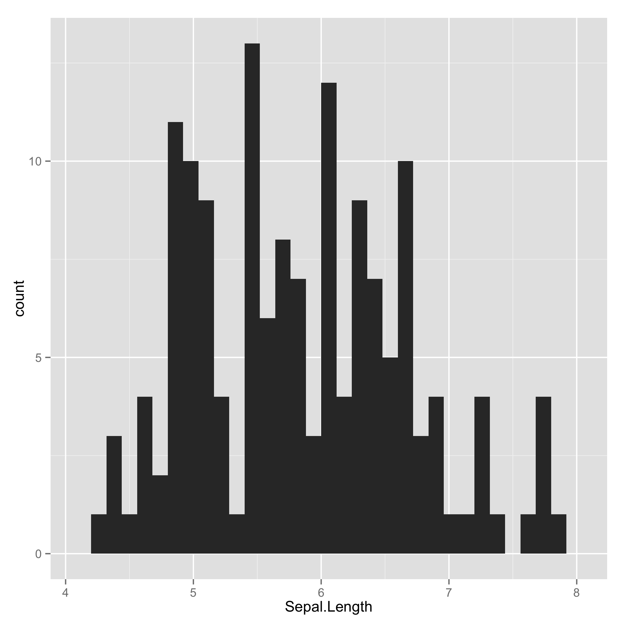
引数に何も取らずにgeom_histogram()を使うと, 上のようなグラフが描写されます.
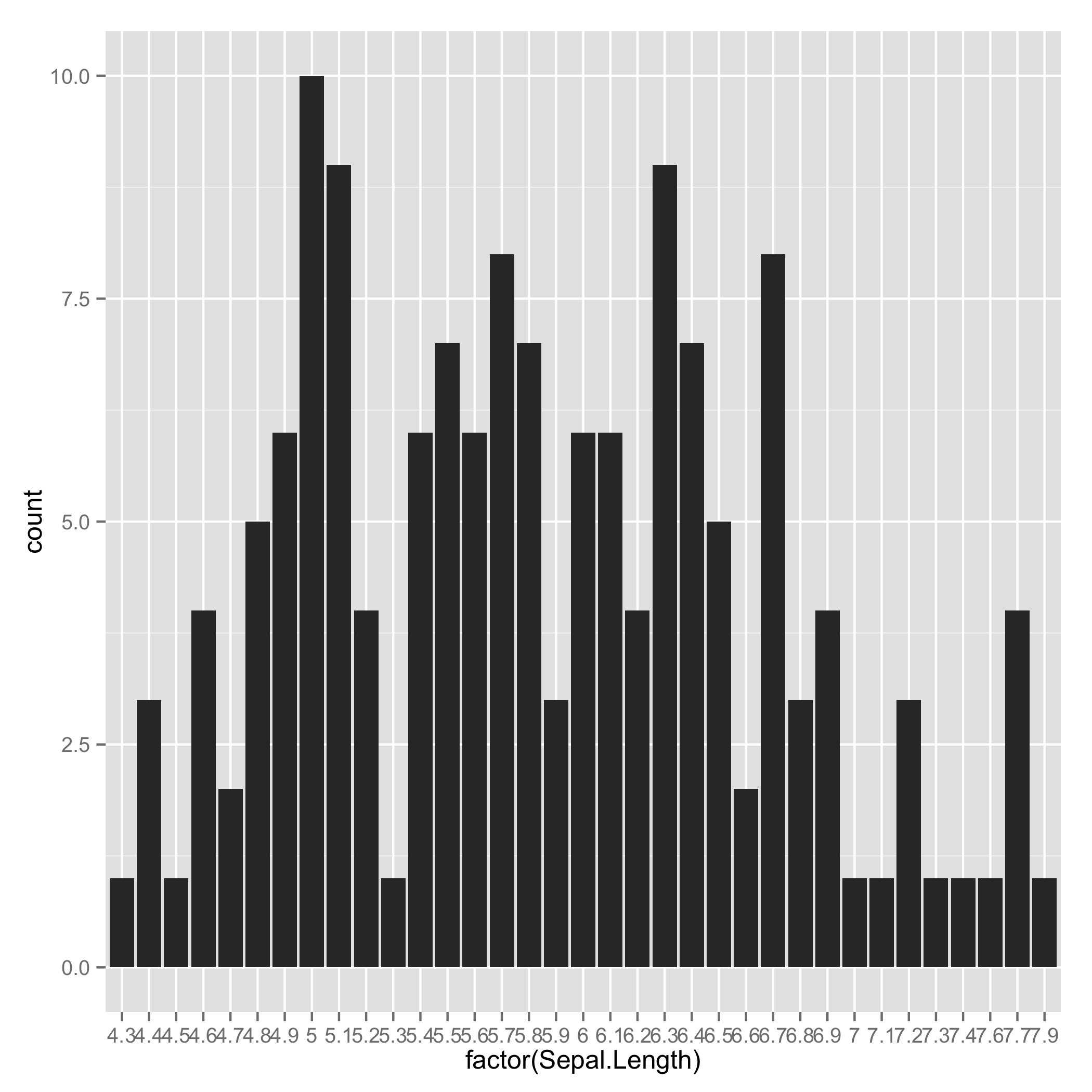
パラメータの値ごとに, 度数を見たいときは, factor()を使って, 以下のようにします.
> p <- ggplot(iris, aes(x=factor(Sepal.Length)))
> p + geom_histogram()
> ggsave("geom_histogram2.png")
Saving 7 x 7 in image
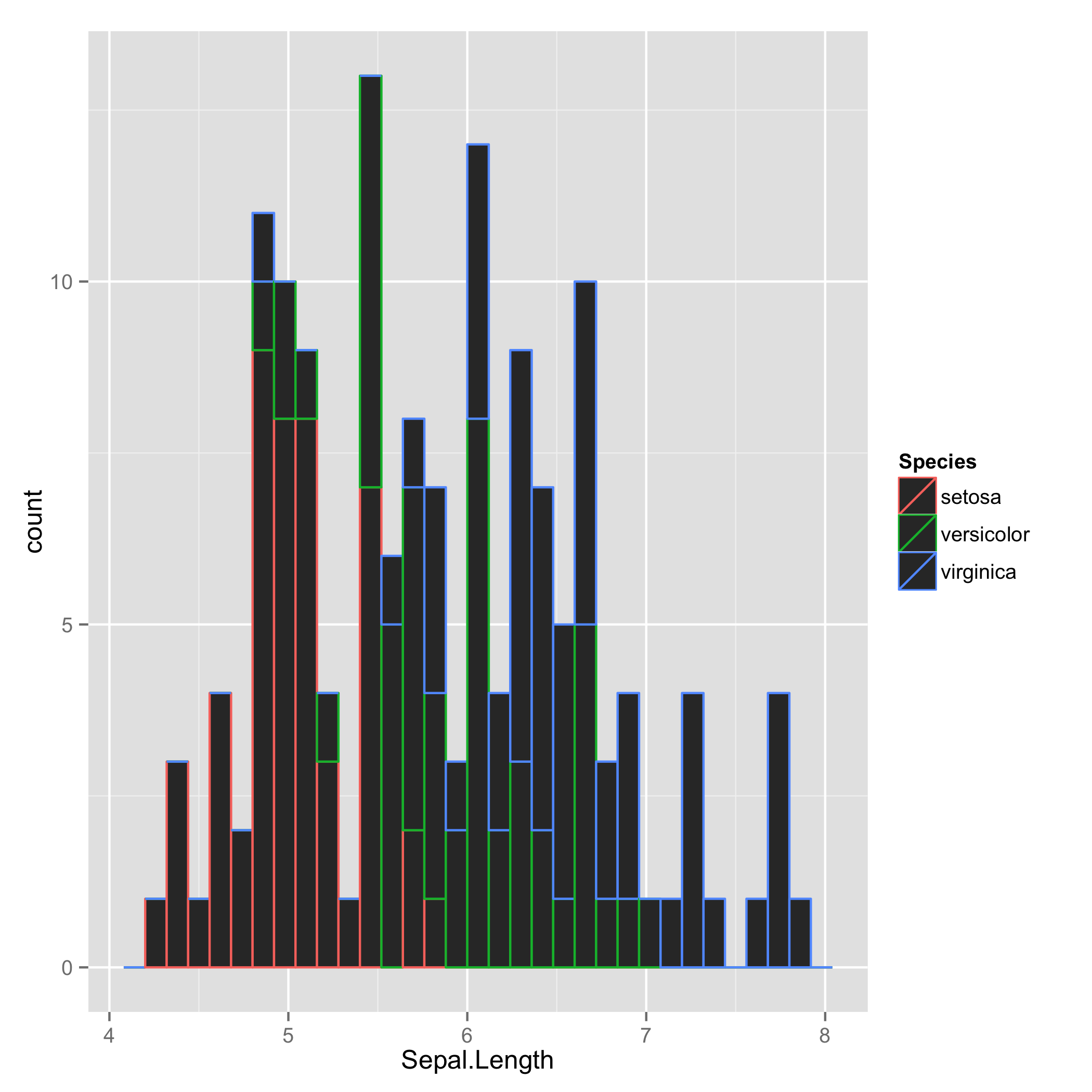
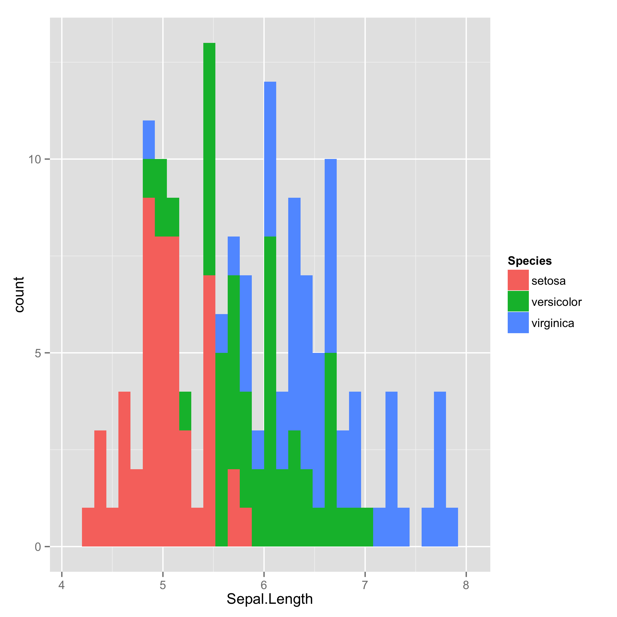
次に, 一番初めのグラフをSpeciesパラメータで色分けをしたいと思います. そのためには, 色分けをSpeciesパラメータについて行うということを以下のように, 明示的に示します. geom_histogram()では, グラフの枠と, 内部の2種類の色分けがあり, 以下のようになります.
> p <- ggplot(iris, aes(x=Sepal.Length))
> p + geom_histogram(aes(colour=Species))
stat_bin: binwidth defaulted to range/30. Use 'binwidth = x' to adjust this.
> ggsave("geom_histogram3.png")
Saving 7 x 7 in image
stat_bin: binwidth defaulted to range/30. Use 'binwidth = x' to adjust this.
>
> p + geom_histogram(aes(fill=Species))
stat_bin: binwidth defaulted to range/30. Use 'binwidth = x' to adjust this.
> ggsave("geom_histogram4.png")
Saving 7 x 7 in image
stat_bin: binwidth defaulted to range/30. Use 'binwidth = x' to adjust this.
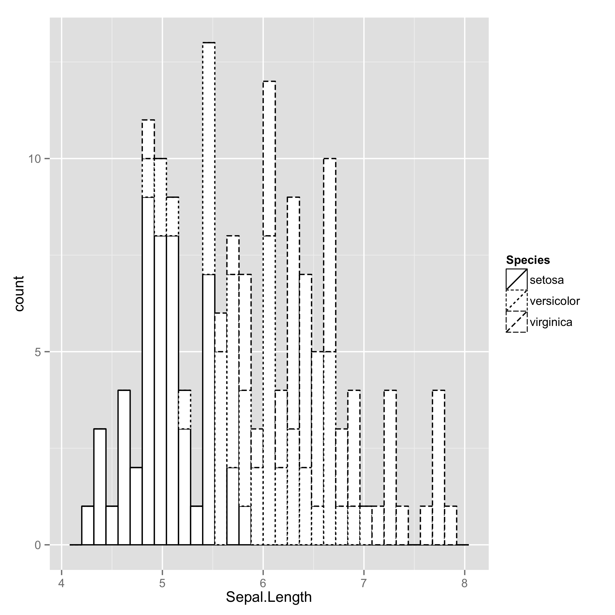
次に, ヒストグラムの枠線の種類を変えてみたいと思います. linetypeというパラメータを使います. 注意としては, 内部のと枠線との色が異なる色でないと, 見えなくなるので注意して下さい. 例では, 枠線の色が黒, 内部の色は白になるように指定します.
> p + geom_histogram(aes(linetype=Species), colour="black", fill="white")
stat_bin: binwidth defaulted to range/30. Use 'binwidth = x' to adjust this.
> ggsave("geom_histogram5.png")
Saving 7 x 7 in image
stat_bin: binwidth defaulted to range/30. Use 'binwidth = x' to adjust this.
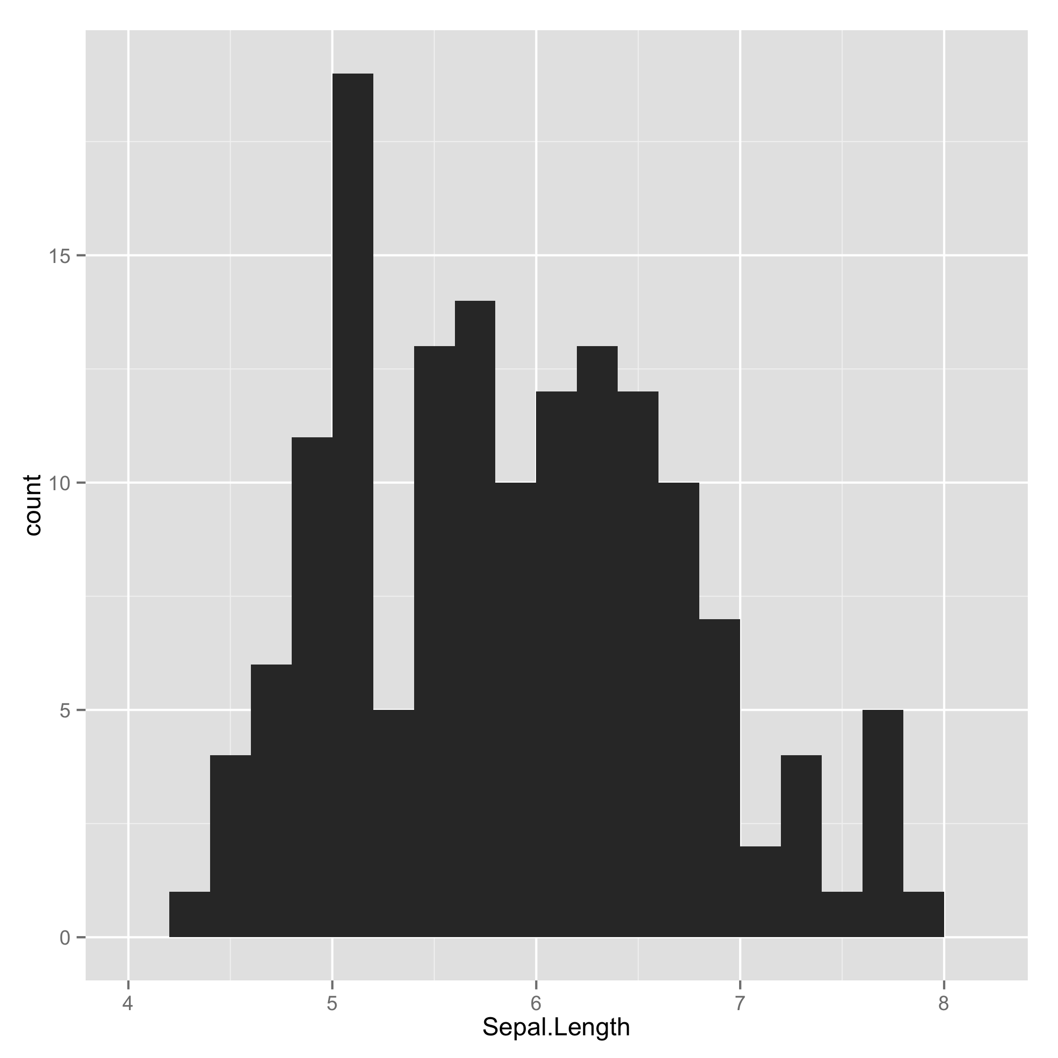
ヒストグラムの1つ1つの棒の幅を変えたいときは, binwidthというパラメータを変更します. 幅を0.2間隔に変えると次にようになります.
> p + geom_histogram(binwidth=0.2)
> ggsave("geom_histogram6.png")
Saving 7 x 7 in image
geom_histogram()の使い方はこんな感じになると思います.